Machine Learning Interview: Sampling and dataset generation
2022-01-17Understanding Jacobian and Hessian matrices with example
2022-03-02When analyzing data within groups, Pyspark window functions can be more useful than using groupBy for examining relationships. First, a window function is defined, and then a separate function or set of functions is selected to operate within that window. Spark SQL has three types of window functions: ranking functions, analytic functions, and aggregate functions. A summary of the available ranking and analytic functions is provided in the table below. For aggregate functions, users can employ any pre-existing aggregate function as a window function.
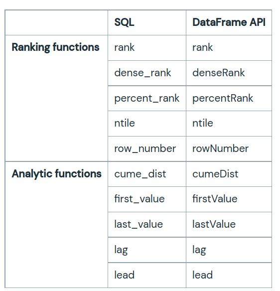
To use window functions, users need to mark that a function is used as a window function by either
- Adding an OVER clause after a supported function in SQL, e.g.
avg(revenue) OVER (...); or - Calling the over method on a supported function in the DataFrame API, e.g.
rank().over(...).
Once a function is marked as a window function, the next key step is to define the Window Specification associated with this function. A window specification defines which rows are included in the frame associated with a given input row. A window specification includes three parts:
- Partitioning Specification: controls which rows will be in the same partition with the given row. If the user wishes to ensure all rows with the same value for a category column are collected to the same machine before ordering and calculating the frame, a partitioning specification is required. If no partitioning specification is given, then all data must be collected to a single machine.
- Ordering Specification: controls the way in which rows within a partition are ordered, determining the position of the given row within its partition.
- Frame Specification: states which rows will be included in the frame for the current input row, based on their relative position to the current row. For instance, “the three rows preceding the current row to the current row” describes a frame containing the current input row and three rows appearing before it.
To specify partitioning expressions for the partitioning specification and ordering expressions for the ordering specification, the SQL keywords PARTITION BY and ORDER BY are employed, respectively. The SQL syntax is illustrated below.
OVER (PARTITION BY ... ORDER BY ...)
In the DataFrame API, we provide utility functions to define a window specification. Taking Python as an example, users can specify partitioning expressions and ordering expressions as follows.
from pyspark.sql.window import Window
windowSpec = \
  Window \
    .partitionBy(...) \
    .orderBy(...)
In addition to the ordering and partitioning, users need to define the start boundary of the frame, the end boundary of the frame, and the type of the frame, which are three components of a frame specification.
There are five types of boundaries, which are UNBOUNDED PRECEDING, UNBOUNDED FOLLOWING, CURRENT ROW, <value> PRECEDING, and <value> FOLLOWING. UNBOUNDED PRECEDING and UNBOUNDED FOLLOWING represent the first row of the partition and the last row of the partition, respectively. For the other three types of boundaries, they specify the offset from the position of the current input row and their specific meanings are defined based on the type of the frame. There are two types of frames: ROW frame and RANGE frame.
ROW frame
ROW frames are based on physical offsets from the position of the current input row, which means that CURRENT ROW, <value> PRECEDING, or <value> FOLLOWING specifies a physical offset. If CURRENT ROW is used as a boundary, it represents the current input row. <value> PRECEDING and <value> FOLLOWING describes the number of rows that appear before and after the current input row, respectively. The following figure illustrates a ROW frame with a 1 PRECEDING as the start boundary and 1 FOLLOWING as the end boundary (ROWS BETWEEN 1 PRECEDING AND 1 FOLLOWING in the SQL syntax).

RANGE frame
RANGE frames are based on logical offsets from the position of the current input row and have a similar syntax to the ROW frame. A logical offset is a difference between the value of the ordering expression of the current input row and the value of that same expression of the boundary row of the frame. Because of this definition, when a RANGE frame is used, only a single ordering expression is allowed. Also, for a RANGE frame, all rows having the same value of the ordering expression with the current input row are considered as the same row as far as the boundary calculation is concerned.
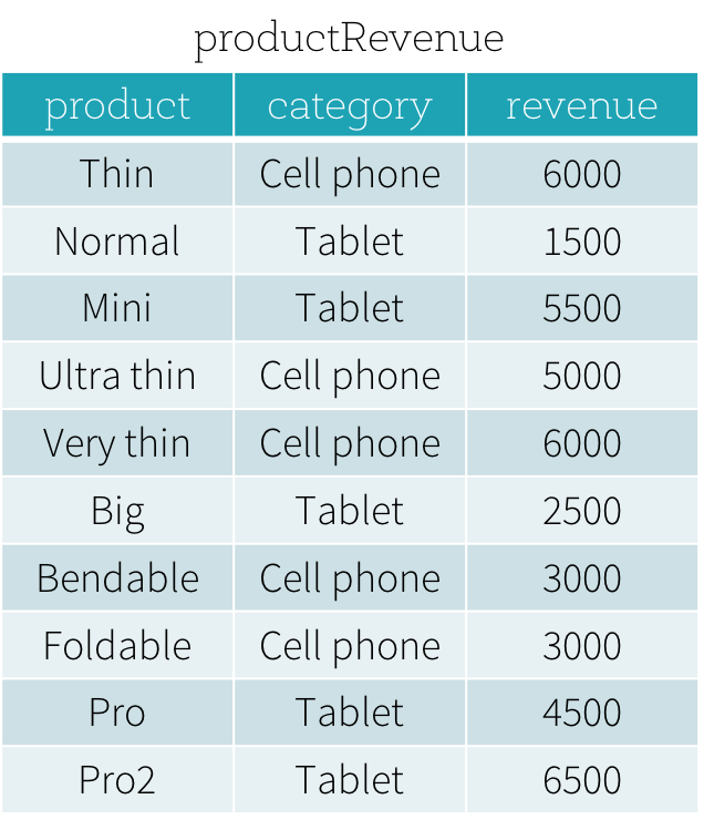
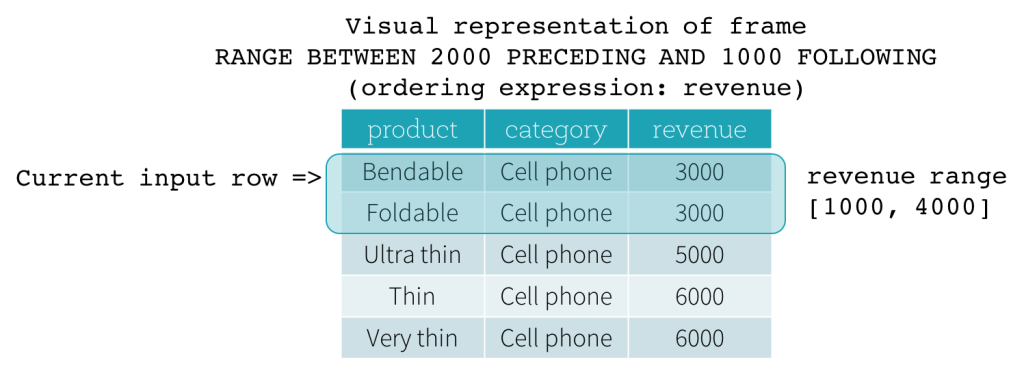
Now, let’s take a look at an example. In this example, the ordering expressions is revenue; the start boundary is 2000 PRECEDING; and the end boundary is 1000 FOLLOWING (this frame is defined as RANGE BETWEEN 2000 PRECEDING AND 1000 FOLLOWING in the SQL syntax). The following five figures illustrate how the frame is updated with the update of the current input row. Basically, for every current input row, based on the value of revenue, we calculate the revenue range [current revenue value - 2000, current revenue value + 1000]. All rows whose revenue values fall in this range are in the frame of the current input row.


In summary, to define a window specification, users can use the following syntax in SQL.
OVER (PARTITION BY ... ORDER BY ... frame_type BETWEEN start AND end)
Here, frame_type can be either ROWS (for ROW frame) or RANGE (for RANGE frame); start can be any of UNBOUNDED PRECEDING, CURRENT ROW, <value> PRECEDING, and <value> FOLLOWING; and end can be any of UNBOUNDED FOLLOWING, CURRENT ROW, <value> PRECEDING, and <value> FOLLOWING.
In the Python DataFrame API, users can define a window specification as follows.
from pyspark.sql.window import Window
# Defines partitioning specification and ordering specification.
windowSpec = \
  Window \
    .partitionBy(...) \
    .orderBy(...)
# Defines a Window Specification with a ROW frame.
windowSpec.rowsBetween(start, end)
# Defines a Window Specification with a RANGE frame.
windowSpec.rangeBetween(start, end)
Examples:
import pandas as pd
import pyspark.sql.functions as fn
from pyspark.sql import SparkSession
from pyspark.sql import Window
# Create a spark session
spark_session = SparkSession.builder.getOrCreate()

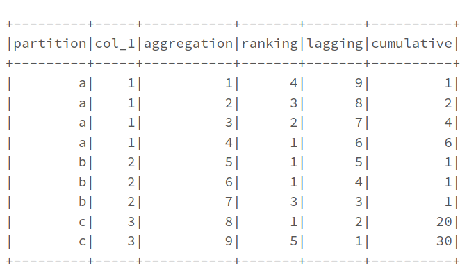
# lets define a demonstration DataFrame to work on
df_data = {'partition': ['a','a', 'a', 'a', 'b', 'b', 'b', 'c', 'c',],
           'col_1': [1,1,1,1,2,2,2,3,3,],
           'aggregation': [1,2,3,4,5,6,7,8,9,],
           'ranking': [4,3,2,1,1,1,3,1,5,],
           'lagging': [9,8,7,6,5,4,3,2,1,],
           'cumulative': [1,2,4,6,1,1,1,20,30,],
          }
df_pandas = pd.DataFrame.from_dict(df_data)
# create spark dataframe
df = spark_session.createDataFrame(df_pandas)
df.show()
Simple aggregation functions
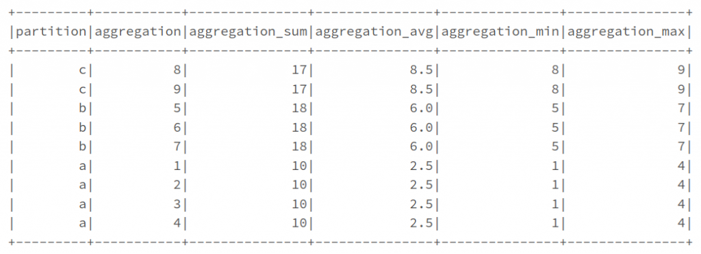
We can use the standard group by aggregations with window functions. These functions use the simplest form of window which just defines a grouping
# aggregation functions use the simplest form of window which just defines grouping
aggregation_window = Window.partitionBy('partition')

# then we can use this window function for our aggregations
df_aggregations = df.select(
  'partition', 'aggregation'
).withColumn(
  'aggregation_sum', fn.sum('aggregation').over(aggregation_window),
).withColumn(
  'aggregation_avg', fn.avg('aggregation').over(aggregation_window),
).withColumn(
  'aggregation_min', fn.min('aggregation').over(aggregation_window),
).withColumn(
  'aggregation_max', fn.max('aggregation').over(aggregation_window),
)

df_aggregations.show()
# note that after this operation the row order of display within the dataframe may have changed
Row-wise ordering and ranking functions
We can also use window functions to order and rank data. These functions add an element to the definition of the window which defines both grouping AND ordering. The function returns the statistical rank of a given value for each row in a partition or group. The goal of this function is to provide consecutive numbering of the rows in the resultant column, set by the order selected in the Window.partition for each partition specified in the OVER clause. E.g. row_number(), rank(), dense_rank(), etc.
# lets define a ranking window
ranking_window = Window.partitionBy('partition').orderBy('ranking')

df_ranks = df.select(
  'partition', 'ranking'
).withColumn(
  # note that fn.row_number() does not take any arguments
  'ranking_row_number', fn.row_number().over(ranking_window)
).withColumn(
  # rank will leave spaces in ranking to account for preceding rows receiving equal ranks
  'ranking_rank', fn.rank().over(ranking_window)
).withColumn(
  # dense rank does not account for previous equal rankings
  'ranking_dense_rank', fn.dense_rank().over(ranking_window)
).withColumn(
  # percent rank ranges between 0-1 not 0-100
  'ranking_percent_rank', fn.percent_rank().over(ranking_window)
).withColumn(
  # fn.ntile takes a parameter for now many 'buckets' to divide rows into when ranking
  'ranking_ntile_rank', fn.ntile(2).over(ranking_window)
)

df_ranks.show()

Creating lagged columns
If we want to conduct operations like calculating the difference between subsequent operations in a group, we can use window functions to create the lagged values we require to perform the calculation. Where there is no preceding lag value, a null entry will be inserted not a zero.
The inverse of lag is lead. Effectively fn.lag(n) == fn.lead(-n)
lag_window = Window.partitionBy('partition').orderBy('lagging')

df_lagged = df.select(
  'partition', 'lagging'
).withColumn(
  # note that lag requires both column and lag amount to be specified
  # It is possible to lag a column which was not the orderBy column
  'lagging_lag_1', fn.lag('lagging', 1).over(lag_window)
).withColumn(
  'lagging_lag_2', fn.lag('lagging', 2).over(lag_window)
).withColumn(
  'lagging_lead_1', fn.lead('lagging', 1).over(lag_window)
).withColumn(
  # note how 'lagging_lag_1' == 'lagging_lead_minus_1'
  'lagging_lead_minus_1', fn.lead('lagging', -1).over(lag_window)
).withColumn(
  # we can also perform calculations between lagged and unlagged columns of course
  'difference_between', fn.col('lagging') - fn.lag('lagging', 1).over(lag_window)
)

df_lagged.show()

Cumulative Calculations (Running totals and averages)
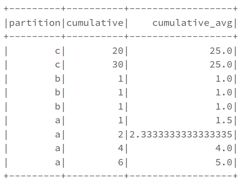
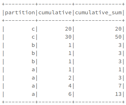
There are often good reasons to want to create a running total or running average column. In some cases, we might want running totals for subsets of data. Window functions can be useful for that sort of thing. In order to calculate such things, we need to add yet another element to the window. Now we account for partition, order, and which rows should be covered by the function. This can be done in two ways we can use rangeBetween to define how similar values in the window must be to be considered, or we can use rowsBetween to define how many rows should be considered. The current row is considered row zero, the following rows are numbered positively and the preceding rows negatively. For cumulative calculations you can define “all previous rows” with Window.unboundedPreceding and “all following rows” with Window.unboundedFolowing
Note that the window may vary in size as it progresses over the rows since at the start and end part of the window may “extend past” the existing rows
#suppose we want to average over the previous, current, and next values
# running calculations need a more complicated window as shown here
cumulative_window_1 = Window.partitionBy(
  'partition'
).orderBy(
  'cumulative'
# for a rolling average lets use rowsBetween
).rowsBetween(
  -1,1
)

df_cumulative_1 = df.select(
  'partition', 'cumulative'
).withColumn(
  'cumulative_avg', fn.avg('cumulative').over(cumulative_window_1)
)

df_cumulative_1.show()
# note how the averages don't use 3 rows at the ends of the window
# running totals also require a more complicated window as here.
cumulative_window_2 = Window.partitionBy(
  'partition'
).orderBy(
  'cumulative'
# in this case we will use rangeBetween for the sum
).rangeBetween(
# In this case we need to use Window.unboundedPreceding to catch all earlier rows
  Window.unboundedPreceding, 0
)

df_cumulative_2 = df.select(
  'partition', 'cumulative'
).withColumn(
  'cumulative_sum', fn.sum('cumulative').over(cumulative_window_2)
)

df_cumulative_2.show()
# note the summing behaviour where multiple identical values are present in the orderBy column
Combining Windows and Calling Different Columns
It is also possible to combine windows and also to call windows on columns other than the ordering column. These more advanced uses can require careful thought to ensure you achieve the intended results:
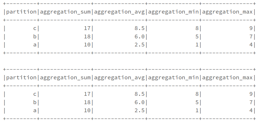
# we can make a window function equivalent to a standard groupBy:
# first define two windows
aggregation_window = Window.partitionBy('partition')
grouping_window = Window.partitionBy('partition').orderBy('aggregation')

# then we can use this window function for our aggregations
df_aggregations = df.select(
  'partition', 'aggregation'
).withColumn(
  # note that we calculate row number over the grouping_window
  'group_rank', fn.row_number().over(grouping_window)
).withColumn(
  # but we calculate other columns over the aggregation_window
  'aggregation_sum', fn.sum('aggregation').over(aggregation_window),
).withColumn(
  'aggregation_avg', fn.avg('aggregation').over(aggregation_window),
).withColumn(
  'aggregation_min', fn.min('aggregation').over(aggregation_window),
).withColumn(
  'aggregation_max', fn.max('aggregation').over(aggregation_window),
).where(
  fn.col('group_rank') == 1
).select(
  'partition',
  'aggregation_sum',
  'aggregation_avg',
  'aggregation_min',
  'aggregation_max'
)

df_aggregations.show()

# this is equivalent to the rather simpler expression below
df_groupby = df.select(
  'partition', 'aggregation'
).groupBy(
  'partition'
).agg(
  fn.sum('aggregation').alias('aggregation_sum'),
  fn.avg('aggregation').alias('aggregation_avg'),
  fn.min('aggregation').alias('aggregation_min'),
  fn.max('aggregation').alias('aggregation_max'),
)

df_groupby.show()
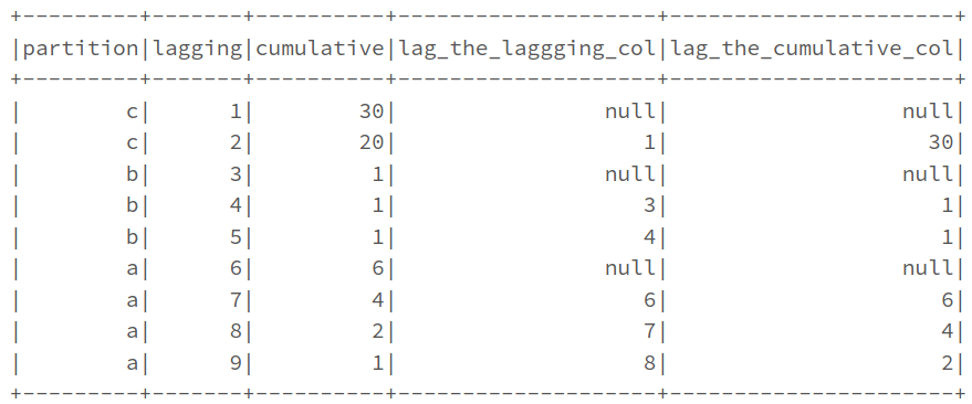
# in some cases we can create a window on one column but use the window on another column
# note that only functions where the column is specified allow this
lag_window = Window.partitionBy('partition').orderBy('lagging')

df_cumulative_2 = df.select(
  'partition', 'lagging', 'cumulative',
).withColumn(
  'lag_the_laggging_col', fn.lag('lagging', 1).over(lag_window)
).withColumn(
  # It is possible to lag a column which was not the orderBy column
  'lag_the_cumulative_col', fn.lag('cumulative', 1).over(lag_window)
)

df_cumulative_2.show()
References:
https://www.geeksforgeeks.org/pyspark-window-functions/
https://sparkbyexamples.com/pyspark/pyspark-window-functions/
https://databricks.com/blog/2015/07/15/introducing-window-functions-in-spark-sql.html

